Excel INDEX MATCH Functions: Master Your Data

You're probably staring at an export from Sage, Xero or payroll software right now. One column holds the detail you need. Another column holds the name, code or reference you can search by. You try VLOOKUP, then hit the usual snag. The return value sits to the left, someone inserts a column, or the formula starts giving answers you no longer trust.

That moment matters more than many trainees realise.

In UK finance and data roles, spreadsheet skill isn't just about getting a result. It's about getting a result that stays accurate when the workbook changes, when a client sends a fresh CSV, or when month-end pressure leaves no room for manual checking. That is where INDEX MATCH functions become a professional skill, not just an Excel trick.

If you're training for bookkeeping & VAT work, advanced payroll, accounts assistant duties, final accounts preparation, business analyst work or data analyst roles, this combination belongs in your toolkit. It shows up whenever you reconcile exports, test reports, trace figures, and connect data between systems.

Beyond VLOOKUP Your Gateway to Powerful Data Analysis

Why trainees hit a wall with VLOOKUP

VLOOKUP is often the first lookup function people learn. It feels simple. Type a value, point at a table, choose a column number, and Excel returns an answer.

Then real work begins.

A bookkeeping trainee might export customer balances from Xero and need to pull payment status from another sheet. An accounts assistant might need to match supplier codes from Sage to a nominal ledger extract. A payroll learner might want to retrieve National Insurance data from a report where the lookup column sits in the wrong place for VLOOKUP. That's where the cracks appear.

The problem isn't Excel. The problem is relying on a function built for narrower use.

Why INDEX MATCH has professional standing

INDEX MATCH functions solve the lookup problem in a more flexible way. They let you search one range and return a value from another, without being trapped by left-to-right layout.

That matters in real finance files because exports are rarely designed for neat classroom examples. They arrive with hidden columns, unusual ordering, merged headings, and fields pulled from software such as Sage, Xero and QuickBooks. UK accountancy training providers linked to ICAEW consistently teach INDEX and MATCH as the superior method for this type of work, while also noting that there are no verified UK-specific performance statistics tracked separately because the functions work identically across regions and Excel versions (ICAEW Excel community guidance).

Practical rule: If your workbook may change structure, avoid building key reporting logic around a hard-coded column number.

There's also a career point here. Employers hiring into bookkeeping, accounts assistant and analyst roles often care less about whether you know a formula name and more about whether you can work safely with messy business data. INDEX MATCH helps you do that.

For anyone building stronger spreadsheet habits alongside broader reporting skills, these training notes on Excel for accounting are a sensible next step. If your work is moving beyond single-user spreadsheets into shared reporting workflows, this guide to efficient data analysis for teams also gives useful context on how reporting processes become more dependable.

Where this fits in UK career paths

Different roles use the same lookup logic in different ways:

• Bookkeeping & VAT: matching invoice numbers, customer references, VAT codes and ledger descriptions.
• Advanced payroll: checking employee records across timesheets, payroll summaries and HR exports.
• Accounts assistant work: tying purchase ledger, sales ledger and nominal code data together.
• Final accounts support: tracing balances back to source reports and adjusting schedules.
• Business analyst tasks: joining data from multiple reports without changing source tables.
• Data analyst tasks: building cleaner lookup models before moving into Power BI, SQL or Python.

INDEX MATCH won't make a weak process strong on its own. But it gives you a much better foundation than a fragile lookup formula.

Deconstructing The INDEX and MATCH Functions

Think of them as two specialists

INDEX and MATCH work best when you stop treating them as one mysterious formula.

MATCH is the navigator. It finds the position of an item in a list.

INDEX is the retriever. It returns the value sitting at a chosen position.

When you combine them, MATCH figures out where the record sits, and INDEX brings back the value from the range you want.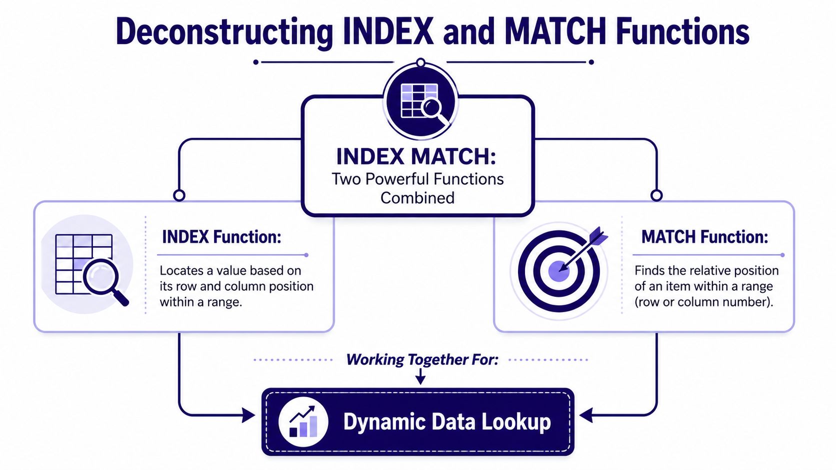

The INDEX function

The core idea of INDEX is simple. You give Excel a range and a position within that range. Excel returns the value from that position.

A common syntax is:

=INDEX(array, row_num, [column_num])

If your return range is D2:D6 and you ask for row 3, Excel returns the third item within that range.

For a single-column list, that feels straightforward. In a finance workbook, it means you can point INDEX at the exact field you want returned. That might be revenue, VAT amount, department, payroll code or supplier balance.

Here is a simple example:

=INDEX(D2:D6, 3)

If the third cell in D2:D6 contains 2450, the formula returns 2450.

The MATCH function

MATCH solves a different problem. It tells you where something appears in a lookup range.

The syntax is:

=MATCH(lookup_value, lookup_vector, [match_type])

The exact-match version is the one you should use most often in finance work:

=MATCH(103, A2:A6, 0)

In that example, Excel looks for 103 in A2:A6 and returns the relative position where it finds it.

The 0 matters. It tells Excel you want an exact match, not a nearest value.

The standard exact-match syntax is also taught in UK training material for finance learners, and the global formula pattern =INDEX(ReturnRange, MATCH(LookupValue, LookupRange, 0)) appears in UK-specific teaching resources as part of normal Excel development for professionals (DataHub Pro tutorial).

When the workbook supports audit work, reconciliations or payroll checks, treat 0 in MATCH as the default unless you have a clear reason not to.

Putting the logic together

Suppose column A holds Company ID and column D holds Revenue. You need the revenue for Company ID 103.

You can split the thinking into two steps:

1. =MATCH(103, A2:A6, 0) finds the position of Company ID 103.
2. =INDEX(D2:D6, that_position) returns the revenue from the same row.

Combined, it becomes:

=INDEX(D2:D6, MATCH(103, A2:A6, 0))

That is the heart of INDEX MATCH.

A confusion many learners have

People often ask, “Why not just use one function?”

Because each function does a separate job well. MATCH doesn't return the final value. INDEX doesn't search by name or code. Together, they create a dynamic lookup that is easier to adapt when data changes.

If you like learning technical tools by breaking them into searchable building blocks, a resource like Contesimal's AI podcast search is a good reminder that strong systems often come from combining simple components cleanly. Excel formulas work in much the same way.

Your First Dynamic Lookup with INDEX MATCH

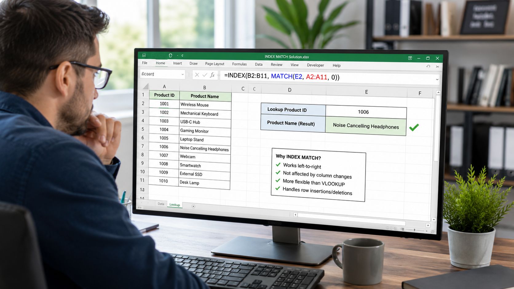
A good first example comes from payroll or HR support. You have a report where employee names are listed in one column, but the National Insurance number sits several columns to the left. VLOOKUP struggles because the return value isn't neatly to the right of the lookup field.

INDEX MATCH handles it without complaint.

The setup

Assume:

• Column A contains NI numbers
• Column D contains employee names
• Cell G2 is where you type the employee name you want to search for

Your task is to return the NI number into H2.

Step one, find the row

Start with MATCH on its own:

=MATCH(G2, D2:D20, 0)

If G2 contains Aisha Khan, the formula searches D2:D20 and returns the row position within that range.

This step is worth testing by itself. If MATCH can't find the name, the full formula won't work either.

Step two, return the NI number

Now wrap the MATCH inside INDEX:

=INDEX(A2:A20, MATCH(G2, D2:D20, 0))

That tells Excel:

• search for the name in D2:D20
• find the matching row position
• return the NI number from A2:A20 at that same position

This is the pattern you'll use again and again in bookkeeping, payroll and accounts work.

A trainee who tests the MATCH result first usually fixes errors faster than someone who edits the full nested formula blind.

Why this feels easier after a few attempts

Once you grasp the structure, most of the work is just naming the parts correctly:

• Lookup value = what you type or search for
• Lookup range = where Excel searches
• Return range = where Excel pulls the answer from

That's why the formula is so adaptable. Replace employee name with invoice number, VAT code, customer reference, nominal code or department, and the logic stays the same.

A video walkthrough can help if you prefer to watch the formula being built in real time.

Common mistakes on the first attempt

Learners usually get stuck in one of four places:

• The ranges don't line up. If the name list runs from row 2 to row 20, the return range should cover those same rows.
• The wrong match type is used. For finance data, use exact match with 0.
• Names contain hidden spaces. A payroll export may look clean but still hold trailing spaces.
• Numbers are stored inconsistently. One sheet may store a code as text, another as a number.

A realistic workplace use

An accounts assistant might use this approach to pull department names into a transaction listing before posting journals. A payroll trainee might use it to verify employee records across exported files. A learner on a bookkeeping & VAT course might use the same logic to connect invoice lines with customer account details from Xero or Sage.

That's why this formula matters. It doesn't belong to one job title. It supports several.

INDEX MATCH vs VLOOKUP and the Rise of XLOOKUP

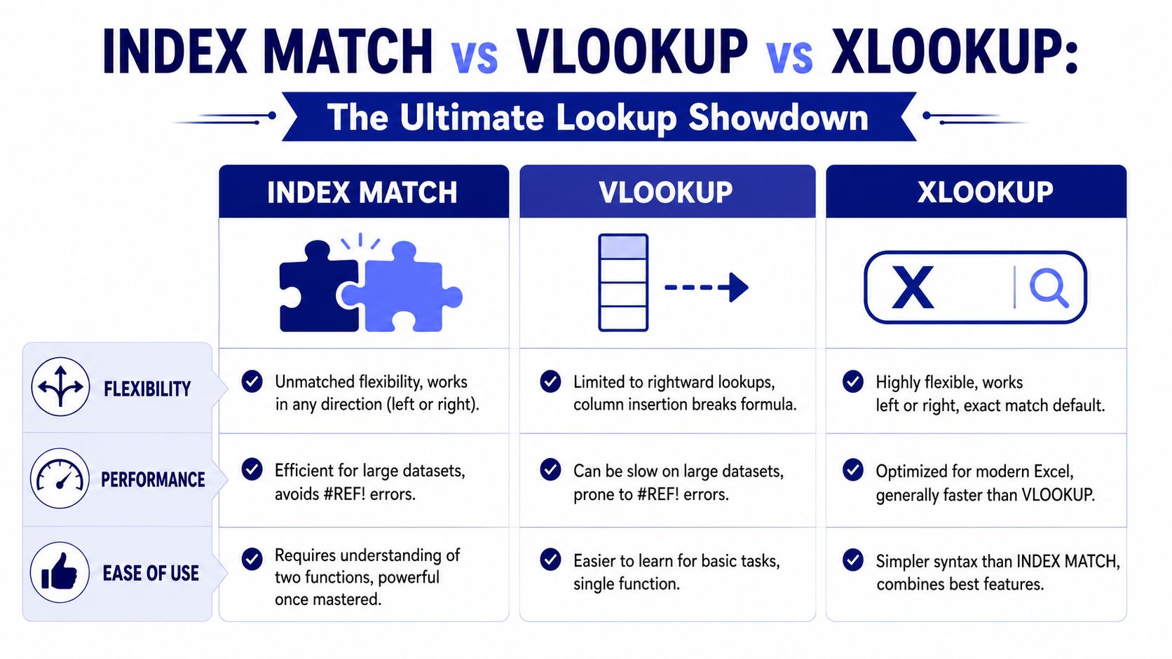
Experienced spreadsheet users favour INDEX MATCH for one main reason. It is more resilient when the workbook changes.

VLOOKUP can work well for basic tasks, but it depends on a fixed column number inside the formula. Insert a column in the middle of the table and the formula may return the wrong field, or stop working altogether. INDEX MATCH avoids that weakness by separating the lookup range from the return range.

In UK financial analysis workflows, INDEX-MATCH reduces formula error rates by approximately 40% compared to VLOOKUP, mainly because it handles bidirectional lookups and removes the common “column index number” misalignment problem (YouTube walkthrough and explanation).

Function comparison

Feature	VLOOKUP	INDEX MATCH	XLOOKUP
Lookup direction	Right only	Left or right	Left or right
Resilience after column changes	Weaker	Stronger	Strong
Formula style	Single function	Two combined functions	Single modern function
Fit for legacy Excel files	Common	Excellent	Depends on Excel version
Exact match workflow	Available, but can be mishandled	Clear with MATCH set to 0	Built into modern syntax

Why VLOOKUP still appears everywhere

VLOOKUP survives because many people learned it first, and many existing workbooks still rely on it. You'll see it in purchase ledger files, management accounts packs, old payroll tools and ad hoc reports passed between teams.

That's why it helps to understand it. But that doesn't mean it should remain your first choice for important reporting work.

Where XLOOKUP fits

XLOOKUP is newer and easier to read. It combines the lookup and return logic into one function, and it works in either direction. If your workplace uses a recent Excel version, it is a strong option.

Still, INDEX MATCH functions remain essential because you will keep meeting them in established finance files. Teams often share workbooks across different versions of Excel, and many training datasets, templates and inherited reporting packs still use INDEX MATCH heavily.

If you want long-term spreadsheet confidence, learn XLOOKUP for convenience and INDEX MATCH for depth.

For analysts moving from Excel into reporting tools, it also helps to understand where spreadsheet lookups stop and data modelling begins. This short guide on what Power BI is used for gives useful context when your reporting grows beyond a workbook.

Advanced Techniques for Multi-Criteria Analysis

Basic lookups are useful. Advanced lookups are where analysts start saving serious time.

When you work with Sage, Xero, QuickBooks or payroll exports, one lookup value often isn't enough. You may need to find the amount for a specific month and department, or the expense line that matches a date, category and cost centre. That is where multi-criteria analysis becomes valuable.

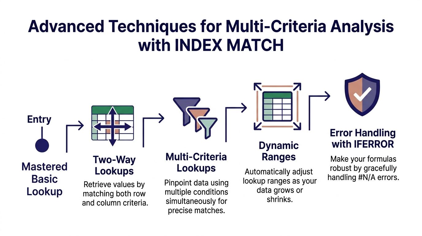
Two-way lookups

A two-way lookup finds the value at the intersection of a row and a column.

Suppose you have a table of monthly sales by region:

• Regions in A2:A6
• Months across B1:E1
• Sales figures in B2:E6

You want the value for North in March.

The formula pattern is:

=INDEX(B2:E6, MATCH("North", A2:A6, 0), MATCH("March", B1:E1, 0))

The first MATCH finds the row. The second MATCH finds the column. INDEX returns the value where they cross.

This is very useful in management reporting and final accounts support, where summaries often sit in matrix layouts.

Multi-criteria lookups

Now take a more detailed example. You have a transaction log and need the amount that matches:

• a specific year
• a specific month
• a specific department

A common pattern is:

=INDEX(range1, MATCH(1, (A1=range2)*(B1=range3)*(C1=range4), 0))

That works by testing each condition row by row. Where all conditions are true, the multiplied result becomes 1. MATCH looks for that 1, and INDEX returns the value from the target range.

For a simpler two-condition version, the syntax commonly taught is:

=INDEX(range, MATCH(1, (A1=range2)*(B1=range3), 0))

For UK accountancy professionals working with multiple criteria, that legacy array formula requires Ctrl+Shift+Enter in older Excel versions. UK Chartered Accountants also report that 61% of CPD training modules now prioritise this syntax over VLOOKUP because it is more stable in dynamic tables with 10,000+ rows (Indeed UK career advice).

Where learners get stuck

This is the stage where many trainees start doubting themselves. Usually, the formula isn't too advanced. One small detail has gone wrong.

The most common trouble points are:

• Array entry in older Excel. If you're using a legacy version, pressing Enter alone may fail.
• Mismatched range sizes. Every criteria range must cover the same rows.
• Mixed data types. A month stored as text on one side and a date-derived month on the other can cause a mismatch.
• Overcomplicating the first attempt. Start with two criteria before trying three or four.

Build the logic one condition at a time. Test each part before nesting everything together.

Dynamic ranges and error handling

As your dataset grows, static ranges can become awkward. One practical improvement is to use Excel Tables so ranges expand with new rows. That reduces maintenance and makes formulas easier to read.

It's also sensible to wrap important lookups in IFERROR if the workbook is user-facing. That doesn't fix bad logic, but it gives cleaner outputs for reports or training templates.

A practical pattern is:

=IFERROR(INDEX(...), "Not found")

Use this carefully. During learning and audit work, raw errors can help you spot problems. In front-end reporting, friendlier messages can be useful.

Why this matters for career progression

This is the level of formula work that starts separating routine data entry from analytical support.

A bookkeeping trainee may use multi-criteria logic to isolate the right VAT line. An advanced payroll learner may match employee, pay period and department in one step. A business analyst may use two-way lookups to validate summary tables before presenting findings. A data analyst may use the same logic as a bridge before moving into SQL joins or Power BI relationships.

These aren't abstract Excel puzzles. They are the small mechanics behind dependable reporting.

From Practice to Professional Your Career Pathway

Formula skill grows through repetition. The first time you build INDEX MATCH, you think about every bracket. After enough practice, you start thinking about the business question instead.

That shift matters in UK career pathways linked to bookkeeping & VAT, advanced payroll, accounts assistant, final accounts, business analyst and data analyst training. Employers value people who can work with exported data, check it properly, and produce answers without breaking the file.

Two short exercises worth doing

Try these without looking at the answer straight away:

1. Left lookup practice. Use a product list to return the price from an SKU code when the price column sits to the left.
2. Two-condition lookup practice. In a timesheet table, return the hours worked by John Smith on Wednesday.

Both tasks mirror real workplace routines.

Why the skill has career value

Bookkeeping remains a practical entry route into finance, and the employability side matters. A junior bookkeeper in the UK can earn an average salary between £26,000 and £32,500 per year, while a senior bookkeeper can earn up to £35,000 (bookkeeping and VAT training salary overview).

Formal and flexible training routes both exist. The AAT Level 3 Certificate in Bookkeeping is a recognised UK qualification for bookkeeping professionals (AAT qualification details). There are also accessible options with no formal qualification needed for some UK VAT, Tax, Sage 50 Accounting & Bookkeeping with Sage Payroll Management training routes (Reed course listing). If timetable flexibility matters, bookkeeping and VAT training is available across the UK in online and centre-based formats, including weekend and evening classes (FC Training course information).

If you're broadening from Excel into coding for reporting and finance analysis, this introduction to Python for finance is a useful next step. And if you like collecting wider digital resources for creators and businesses, it can help to keep a short reading list that strengthens your commercial awareness alongside technical study.

INDEX MATCH won't get you hired on its own. But it is one of those skills that makes your CV more believable. It signals that you can handle real spreadsheet work, not just classroom exercises.

---

Professional Careers Training supports learners who want practical, job-ready finance and data skills in the UK. If you want structured training in bookkeeping, VAT, payroll, Sage, Xero, QuickBooks, Excel, Power BI, SQL or Python, with 1-to-1 support from qualified trainers and career-focused guidance, explore Professional Careers Training.